强化学习之ConnectX四子棋游戏

Connect X

Time: 2022.11.14

Author: Shaw

Connect X | Kaggle

ConnectX Getting Started | Kaggle

一、任务简介：

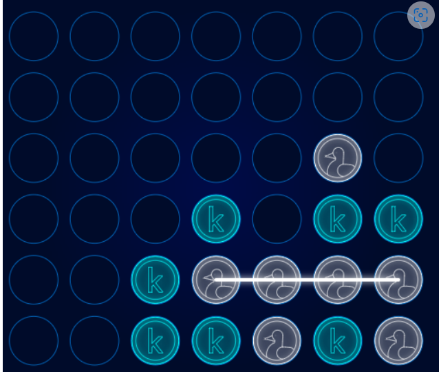
• 任务：强化学习任务，类似五子棋的规则（但每一步只能下某一列的最底端的空位），每人一步，先于对手横竖或斜角连成4个即可获胜。

• 评估方法：

  每个提交给Kaggle的结果（一个py文件，包含了agent如何下棋的规则）在跟自己下一次棋，证明其工作正常后，会被赋予一个skill等级。

  相近skill等级的提交结果之间会进行持续不断下棋PK。

  每次PK结束后就会更新双方的等级，赢加输减。

二、环境准备

安装kaggle相关的强化学习环境：

pip install kaggle-environments

创建Connect X环境：

from kaggle_environments import evaluate, make, utils

env = make("connectx",debug=True)   #创建connectx环境
env.render()                        #以图形化的形式显示当前环境

创建Submission提交函数：

import inspect
import os

def write_agent_to_file(function, file):
    with open(file, "a" if os.path.exists(file) else "w") as f:
        f.write(inspect.getsource(function))
        print(function, "written to", file)

write_agent_to_file(my_agent, "submission.py")

三、Q-learning

对于简单的下棋问题，这里选择Q-learning算法进行学习。

创建connectX类：

class ConnectX(gym.Env):
    def __init__(self, switch_prob=0.5):
        self.env = make('connectx', debug=True)
        self.pair = [None, 'negamax']
        self.trainer = self.env.train(self.pair)
        self.switch_prob = switch_prob
        
        # Define required gym fields (examples):
        config = self.env.configuration
        self.action_space = gym.spaces.Discrete(config.columns)
        self.observation_space = gym.spaces.Discrete(config.columns * config.rows)

    def switch_trainer(self):
        self.pair = self.pair[::-1]
        self.trainer = self.env.train(self.pair)

    def step(self, action):
        return self.trainer.step(action)
    
    def reset(self):							# 有switch_prob的几率更换先手顺序
        if random.uniform(0, 1) < self.switch_prob:
            self.switch_trainer()
        return self.trainer.reset()
    
    def render(self, **kwargs):
        return self.env.render(**kwargs)

创建Q表，由于棋盘状态较多，这里使用动态Q表（shape = （n，7））：

class QTable:
    def __init__(self, action_space):
        self.table = dict()
        self.action_space = action_space

    def add_item(self, state_key):
        self.table[state_key] = list(np.zeros(self.action_space.n))

    def __call__(self, state):
        board = state['board'][:]  				# 复制一份
        board.append(state.mark) 					# 加入mark标志着先手还是后手
        state_key = np.array(board).astype(str)	
        state_key = hex(int(''.join(state_key), 3))[2:]# 转为16进制编码，去掉前缀
        if state_key not in self.table.keys():
            self.add_item(state_key)

        return self.table[state_key]

定义相关超参数：

alpha = 0.1				# 学习率
gamma = 0.6				# discount factor γ
epsilon = 0.99				# ε-greedy策略的ε
min_epsilon = 0.1			# 最小ε

episodes = 10000			# 采样轮数

alpha_decay_step = 1000
alpha_decay_rate = 0.9		# α衰减率
epsilon_decay_rate = 0.9999	# ε衰减率

定义训练过程：

q_table = QTable(env.action_space)

all_epochs = []
all_total_rewards = []
all_avg_rewards = [] # Last 100 steps
all_qtable_rows = []
all_epsilons = []

for i in tqdm(range(episodes)):
    state = env.reset()     # 清空棋盘
    epochs,total_rewards = 0, 0
    epsilon = max(min_epsilon,epsilon*epsilon_decay_rate)   # ε每轮衰减
    done = False

    while not done :    # 开始一轮采样
        # 某列不能下的情况 == 此列的第一个位置有棋子 == (state.board[c] == 0)
        space_list = [c for c in range(env.action_space.n) if state['board'][c] == 0]

        if random.uniform(0,1) <= epsilon :# ε-greedy-->选择随机策略
            action = choice(space_list)
        else : 					   # ε-greedy-->选择贪心策略
            row = np.array(q_table(state)[:])
            row[[c for c in range(env.action_space.n)
                 if state['board'][c] != 0]] = -1
            action = int(np.argmax(row))
        
        next_state,reward,done,info = env.step(action)

        if done:
            if reward == 1: # Won
                reward = 20
            elif reward == 0: # Lost
                reward = -20
            else: 
                reward = 1
        else:
            reward = -0.01

        old_value = q_table(state)[action]
        next_max = np.max(q_table(next_state))
	   # Q-Learning 更新
        new_value = (1 - alpha) * old_value + alpha * (reward + gamma * next_max)
        q_table(state)[action] = new_value

        state = next_state
        epochs += 1
        total_rewards += reward

    all_epochs.append(epochs)
    all_total_rewards.append(total_rewards)
    avg_rewards = np.mean(all_total_rewards[max(0, i-100):(i+1)])
    all_avg_rewards.append(avg_rewards)
    all_qtable_rows.append(len(q_table.table))
    all_epsilons.append(epsilon)

    if (i+1) % alpha_decay_step == 0:
        alpha *= alpha_decay_rate

根据Q表生成Agent：

my_agent = '''def my_agent(observation, configuration):
    from random import choice

    q_table = ''' \
    + str(dict_q_table).replace(' ', '') \
    + '''

    board = observation.board[:]
    board.append(observation.mark)
    state_key = list(map(str, board))
    state_key = hex(int(''.join(state_key), 3))[2:]

    if state_key not in q_table.keys():
        return choice([c for c in range(configuration.columns) if observation.board[c] == 0])

    action = q_table[state_key]

    if observation.board[action] != 0:
        return choice([c for c in range(configuration.columns) if observation.board[c] == 0])

    return action
    '''
    
with open('submission.py', 'w') as f:
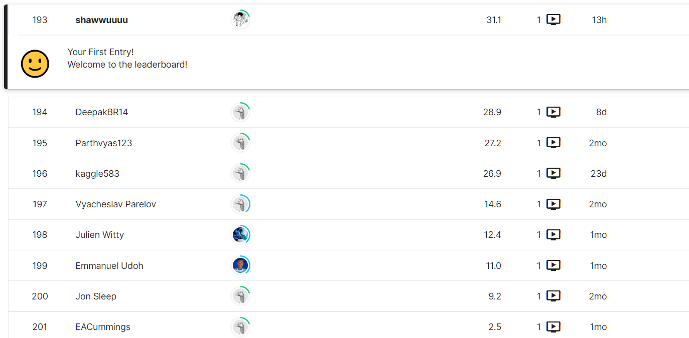
    f.write(my_agent)

上交到Kaggle后经过一晚上的博弈，分数很低，直接倒数：

尝试评估其效果：

from submission import my_agent

def mean_reward(rewards):
    win = sum(1 if r[0]>0 else 0 for r in rewards)
    loss = sum(1 if r[1]>0 else 0 for r in rewards)
    draw = sum(1 if r[0] == r[1] else 0 for r in rewards)
    return '{0} episodes- won: {1} | loss: {2} | draw: {3} | winning rate: {4}%'.format(
        len(rewards),
        win,
        loss,
        draw,
        (win / len(rewards))*100
    )

# Run multiple episodes to estimate agent's performance.
print("My Agent vs Random Agent:", mean_reward(
    evaluate("connectx", [my_agent, "random"], num_episodes=100)))
print("My Agent vs Negamax Agent:", mean_reward(
    evaluate("connectx", [my_agent, "negamax"], num_episodes=100)))

四、DQN

在尝试了简单的强化学习算法后，这里将深度学习与强化学习结合起来，用DQN进行训练：

DQN使用了神经网络来代替Q表，使用函数替代表格，以此解决Q表过大的问题：

class ConnectX(gym.Env):
    def __init__(self, switch_prob=0.5):
        self.env = make('connectx', debug=False)
        self.pair = [None, 'random']
        self.trainer = self.env.train(self.pair)
        self.switch_prob = switch_prob

        # Define required gym fields (examples):
        config = self.env.configuration
        self.action_space = gym.spaces.Discrete(config.columns)
        self.observation_space = gym.spaces.Discrete(config.columns * config.rows)

    def switch_trainer(self):
        self.pair = self.pair[::-1]
        self.trainer = self.env.train(self.pair)

    def step(self, action):
        return self.trainer.step(action)
    
    def reset(self):
        if np.random.random() < self.switch_prob:
            self.switch_trainer()
        return self.trainer.reset()
    
    def render(self, **kwargs):
        return self.env.render(**kwargs)

class DeepModel(torch.nn.Module):
    def __init__(self,num_states,hidden_units,num_actions):
        super(DeepModel,self).__init__()
        self.hidden_layers = nn.ModuleList([])
        for i in range(len(hidden_units)):
            if i == 0:
                self.hidden_layers.append(nn.Linear(num_states,hidden_units[i]))
            else :
                self.hidden_layers.append(nn.Linear(hidden_units[i-1],hidden_units[i]))
        self.output_layers = nn.Linear(hidden_units[-1],num_actions)

    def forward(self,x):
        for layer in self.hidden_layers:
            x = torch.sigmoid(layer(x))
        x = self.output_layers(x)
        return x

class DQN:
    def __init__(self,num_states,num_actions,hidden_units,gamma,max_experiences,min_experiences,batch_size,lr):

        self.num_actions = num_actions
        self.batch_size = batch_size
        self.gamma = gamma
        self.model = DeepModel(num_states,hidden_units,num_actions)
        self.optimizer = optim.Adam(self.model.parameters(), lr = lr)
        self.criterion = nn.MSELoss()
        self.experience = {'s':[],
                           'a':[],
                           'r':[],
                           's2':[],
                           'done':[]
                          }
        self.max_experiences = max_experiences
        self.min_experiences = min_experiences

    def preprocess(self, state):
        result = state.board[:]
        result.append(state.mark)
        return result

    def predict(self,inputs):
        return self.model(torch.from_numpy(inputs).float())

    def train(self,TargetNet):
        if len(self.experience['s']) < self.min_experiences:
            return 0

        ids = np.random.randint(low=0, high=len(self.experience['s']), size=self.batch_size)
        states = np.asarray([self.preprocess(self.experience['s'][i]) for i in ids])
        actions = np.asarray([self.experience['a'][i] for i in ids])
        rewards = np.asarray([self.experience['r'][i] for i in ids])
        states_next = np.asarray([self.preprocess(self.experience['s2'][i]) for i in ids])
        dones = np.asarray([self.experience['done'][i] for i in ids])

        value_next = np.max(TargetNet.predict(states_next).detach().numpy(), axis=1)
        actual_values = np.where(dones, rewards, rewards+self.gamma*value_next)

        actions = np.expand_dims(actions, axis=1)
        actions_one_hot = torch.FloatTensor(self.batch_size, self.num_actions).zero_()
        actions_one_hot = actions_one_hot.scatter_(1, torch.LongTensor(actions), 1)
        selected_action_values = torch.sum(self.predict(states) * actions_one_hot, dim=1)
        actual_values = torch.FloatTensor(actual_values)

        self.optimizer.zero_grad()
        loss = self.criterion(selected_action_values, actual_values)
        loss.backward()
        self.optimizer.step()

    def get_action(self,state,epsilon):
        if np.random.random() < epsilon:
            return int(np.random.choice([c for c in range(self.num_actions) if state.board[c] == 0]))
        else :
            prediction = self.predict(np.atleast_2d(self.preprocess(state)))[0].detach().numpy()
            for i in range(self.num_actions):
                if state.board[i] != 0:
                    prediction[i] = -1e7
            return int(np.argmax(prediction))

    def add_experience(self, exp):
        if len(self.experience['s']) >= self.max_experiences:
            for key in self.experience.keys():
                self.experience[key].pop(0)
        for key, value in exp.items():
            self.experience[key].append(value)

    def copy_weights(self, TrainNet):
        self.model.load_state_dict(TrainNet.state_dict())

    def save_weights(self, path):
        torch.save(self.model.state_dict(), path)

    def load_weights(self, path):
        self.model.load_state_dict(torch.load(path))

训练时，将采样的s,r,a,s’存储下来，等到积累到一定数量后再以batch的形式输入神经网路（这里是全连接层），训练，测试。

通过这种方式，可以极大的增加训练的轮数，这里尝试十万轮（训练时间四小时）：

五、RollOut

RollOut算法是典型的决策时规划算法，其思路是：

1. 对当前状态S的所有可能取值，模拟计算若干次，取得每个的平均Reward；
2. 选取Reward最大的动作A；

模拟计算时使用的策略称之为rollout策略，这里直接采用随机策略。

使用如下类进行蒙特卡洛采样：

class MonteCarlo:
    def __init__(self, env, gamma, episodes):
        '''
        env是当前需要进行模拟采样的状态
        gamma用于计算Reward
        episodes是每个(s,a)的采样次数
        '''
        self.state = deepcopy(env)
        self.all_rewards = [0, 0, 0, 0, 0, 0, 0]
        self.gamma = gamma
        self.episodes = episodes
    def rollout(self, env):
        # 对当前状态进行rollout采样
        mean_reward = 0
        ini_state = env.env.state[0]['observation']
        for i in range(self.episodes):
            r = 0
            gamma = 1
            env.set_state(ini_state)
            state = deepcopy(ini_state)
            done = False
            while not done:
                space_list = [c for c in range(7) if state['board'][c] == 0]
                action = choice(space_list)
                next_state, reward, done, info = env.step(action)
                if done:
                    if reward == 1:
                        r += 20*gamma
                    elif reward == 0:
                        r -= 20*gamma
                    else:
                        r += 1*gamma
                    mean_reward += r
                else:
                    r -= 0.05*gamma
                gamma *= self.gamma
                state = next_state
        return mean_reward/self.episodes

因为MC采样需要在采样后将环境状态恢复，故在原本的ConnectX类中添加设置状态方法，并删除swicth_trainer：

class ConnectX(gym.Env):
    def __init__(self, switch_prob=0.5):
        self.env = make('connectx', debug=True)
        self.pair = [None, 'random']
        self.trainer = self.env.train(self.pair)
        self.switch_prob = switch_prob
        config = self.env.configuration
        self.action_space = gym.spaces.Discrete(config.columns)
        self.observation_space = gym.spaces.Discrete(
            config.columns * config.rows)

    def step(self, action):
        return self.trainer.step(action)

    def set_state(self, init_state):
        self.env.reset()
        self.env.state[0]['observation'] = deepcopy(init_state)

    def reset(self):
        return self.trainer.reset()

    def render(self, **kwargs):
        return self.env.render(**kwargs)

调试时设置play函数：

def play(num,env,gamma,episodes):
    result = {'win':0,'loss':0,'draw':0}
    for i in range(num):
        #print('[GAME{}]:'.format(i))
        done = False
        state = env.reset()
        while not done:
            ini_state = env.env.state[0]['observation']
            space_list = [c for c in range(7) if ini_state['board'][c] == 0]
            R = []
            for action in space_list:  # rollout模拟采样
                env.set_state(ini_state)
                next_state, reward, done, info = env.step(action)
                mc = MonteCarlo(env, gamma, episodes)
                reward = reward + gamma*mc.rollout(env)
                R.append(reward)

            Action = int(np.argmax(R))  # 根据采样结果选择动作

            env.set_state(ini_state)
            next_state, reward, done, info = env.step(Action)

            #print('R = ', R)
            #print('Action = ', Action)
            #print(env.render(mode="ansi"))

            if done:
                if reward == 1:  # Won
                    result['win'] += 1
                    #print('you win!')
                elif reward == 0:  # Lost
                    result['loss'] += 1
                    #print('you loss!')
                else:
                    result['draw'] += 1
                    #print('draw!')
    print('My Agent vs Random Agent:', '{0} episodes- won: {1} | loss: {2} | draw: {3} | winning rate: {4}%'.format(
        num,
        result['win'],
        result['loss'],
        result['draw'],
        (result['win'] / num)*100
    ))
                

六、问题总结

1. 训练时间过长

以Q-Learning为例，一个10000个episodes的训练要耗时2小时+，对于一个简单的四子棋过于耗时。

尝试：

• 尝试在python文件中而不是jupter中训练：训练总时间减少了约2/5，有一定效果；
• 使用DQN时训练速度明显大于Q-leraning（训练十万轮耗时3小时40分钟），猜想可能是神经网络可以使用GPU加速，‘查表’速度更快；

2. Q-Learning训练效果不佳

在经过10000个episode训练后，Q-Learning的表现如下：

通过如下的代码，你可以跟自己的agent下一局，可以发现，经过一万轮训练后的Agent棋力很一般，新手人类也能轻松胜利：

while not done:
    sys.stdout.flush()
    print(env.render(mode="ansi"))
    action = int(input('Input your action:(0-6)'))

    next_state, reward, done, info = env.step(action)

    if done:
        if reward == 1: # Won
            print('you win!')
        elif reward == 0: # Lost
            print('you loss!')
        else: 
            print('draw!')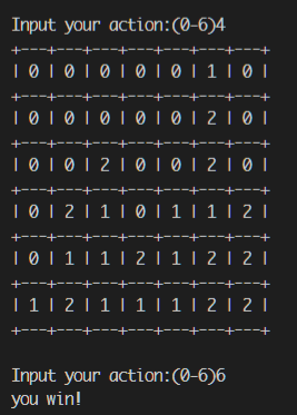

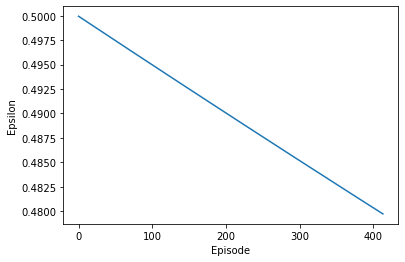
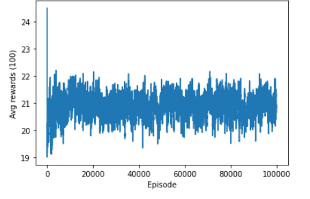
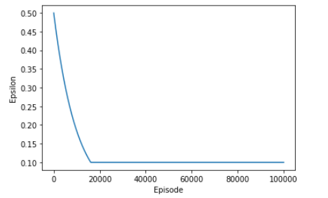
观察训练时平均Reward、Q表长度和ε的变化：

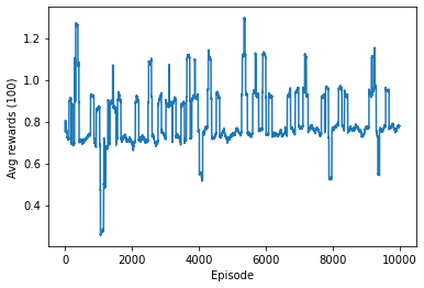
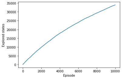
可以发现，在10000轮episode的训练中，平均奖励始终在围绕0.8上下波动，Q表长度一直在平稳增加，这说明直到训练结束Agent仍有大量未见过的state进入Q表，模型训练轮数不足。

实际上 Connect 4有四百万兆不同的状态，Q-learning显然在有限的时间空间下是取得不了什么有效学习的。

3. DQN的不足

即使使用DQN进行了十万轮的训练，耗时近4小时，DQN的结果仍不理想：

其实不难理解，对于四百万兆个state的棋盘，十万轮也不过是$1/10^{13}$，仍过于渺小。

并且，Q-learning以及DQN都是background planning，其算法倾向于将所有可能的状态的最佳策略都计算出来。实际上，在下棋的时候几乎绝大多数状态都不会出现第二次，但相似的棋谱格局却会经常出现。

显然，相较于background planning，decision-time planning（决策时规划）算法是个更合适的算法。

decision-time planning在遇到每个新的状态St后再开始一个完整的规划过程，其为每个当前状态选择一个动作At，到下一个状态St+1就选择一个动作At+1，以此类推。基于当前状态所生成的values和policy会在做完动作选择决策后被丢弃，在很多应用场景中这么做并不算一个很大的损失，因为有非常多的状态存在，且不太可能在短时间内回到同一个状态，故重复计算导致的资源浪费会很少。

4. 随机Rollout

这里尝试使用简单的RollOut算法后发现，即使在rollout算法中使用最简单的随机rollout策略，并且每轮模拟仅仅采样1次，所取得的的结果就比训练了4个小时的DQN好很多。

在模拟采样轮数为1（对每个键值对只采样1次）、gamma为1的条件下，与Random和Negmax分别下100局的胜率：

模型	VS Random	VS Negmax
Q-Learning(一万轮)	61%	3%
DQN(十万轮)	70%	6%
随机Rollout	94%	95%平局

但Rollout算法的问题也很明显，其应用的过程就是‘训练’的过程，每次需要等模拟采样完成后再选择，故其反应时间会比DQN长很多。

时间	DQN	随机Rollout
训练所需时间	4h	0
下100局所需时间	1m	40m

但即使这样，我们也能看出，决策时规划比后台规划算法更适合棋类场景，由于棋类几乎无限的状态数量，决策时规划虽然反应更慢，但结果也更为合理有效。

5. 展望

本次的小比赛从最简单的Q-Learning算法入手，到引入了神经网络的DQN，最后从后台规划引入到决策时规划，并实现了一个简单的Rollout算法。

首先，Q-learning以及DQN这类后台规划算法无法有效处理状态过多的环境。Q-learning在时间以及空间上都存在溢出问题，DQN虽然引入了深度神经网络来替代Q表，解决了空间不足的问题，但由于其训练速度没有质的改变，训练时间仍不可估量的长。

决策时规划面对状态过多的问题有明显提升。即使在rollout算法中使用最简单的随机rollout策略，并且每轮模拟仅仅采样1次，所取得的的结果就比训练了4个小时的DQN好很多。

除了使用简单的随机Rollout算法，这里可以替换rollout策略来进一步提升结果，减少rollout的反应时间。以及，可以使用MCTS，蒙特卡洛树搜索的方法再进一步提升结果（kaggle中已有Notebook，且分数不错），这里篇幅以及时间有限，仅做展望。